Data-driven Design of Autonomous Systems
Introduction
This book is a consolidation of foundations and algorithms for data-driven autonomous system design. The material is distilled from key reference texts in Machine Learning and Robotics.
The material presented is NOT original.
Outline
The content is organized into three parts: Core Math, Applied Theory and Practical Challenges.
I. Mathematics for Autonomous Systems
The foundational theory and reasoning that enables modeling, analyzing and designing autonomous systems.
II. Algorithms and Applications
The theory is only useful when it can be applied to existing problems.
III. Computer Architecture and Bare-Metal Programming
An introductory approach to advanced embedded system development.
Mathematics for Autonomous Systems
This section is intended for robotics engineers and software developers requiring a rigorous framework for autonomous behavior. The following modules cover the core disciplines of Dynamical Systems, Linear Algebra, and Lie Theory, alongside modern approaches in Optimization and Machine Learning. This curriculum establishes the formal language necessary to model physical constraints and manage environmental uncertainty. Mastery of these subjects is a prerequisite for designing and implementing high-performance algorithms for perception, estimation, and real-time motion planning.
%% TITLE: FIGURE 1: Simplified Robotics Domain Map
graph LR
%% Define Node Styles
classDef subject fill:#000000,stroke:#333,stroke-width:2px,rx:5,ry:5,color:#fff;
classDef hub fill:#212121,stroke:#000,stroke-width:3px,rx:10,ry:10,font-weight:bold;

%% 1. The Math Basics
subgraph Foundations
    DS[Dynamical Systems]:::subject
    LS[Linear Systems]:::subject
    PROB[Probability]:::subject
    NUM[Numerical Methods]:::subject
end

%% 2. The Advanced Toolset
subgraph Advanced Topics
    OPT[Optimization]:::subject
    LIE[Lie Theory]:::subject
    ML[Machine Learning]:::subject
end

%% 3. The Robotic Capabilities
subgraph Applications
    EST(Estimation):::hub
    PLAN(Planning):::hub
    PERC(Perception):::hub
    DEC(Decision Making):::hub
end
Outline
Dynamical Systems
Linear and nonlinear ordinary differential equations; Initial Value Problems and numerical integration; Phase Portraits and Equilibrium points; Laplace and Z-transforms; Transfer Functions; effects of poles and zeros on frequency, and stability analysis.
Systems theory provides the mathematical infrastructure for modeling and analyzing systems.
- Inverted Pendulum Simulation: Derive the equations of motion using Lagrangian mechanics and simulate the nonlinear system. Linearize around the upright/downright equilibrium points to analyze their stability.
- Robot Chassis Simulation: Develop a mobile robot chassis model. Start with known constraints (size, weight,...) and then design the parameters of the motors and wheels.
- Frequency Response Analysis: Tune a generic 2nd order transfer function to fit the bode plot of an "unknown" system.
Linear Systems
Vector spaces and norms; matrices and linear transformations; rank, nullity, and the four fundamental subspaces; eigenvalues and eigenvectors; diagonalization and Jordan normal form; orthogonality and projections; least-squares fitting; determinants and inverses; QR, SVD, and LU decompositions; condition numbers and numerical stability.
Nearly every algorithm in robotics reduces to a linear algebra operation. You cannot design a Kalman filter, invert kinematics, optimize trajectories, or compress data without it.
- Camera Calibration: Recover intrinsic and extrinsic parameters from checkerboard images via least-squares regression.
- Dynamic Mode Decomposition: Recover the discrete linear dynamics of a system by exciting it and measuring the states.
- Hardware Optimized BLAS: Implement a custom matrix multiplication function that utilizes a SIMD or NEON hardware feature. Use this function to simulate and analyze a system. Examine the precision and performance between a naive gemm function and a parallelized one.
Probability and Information Theory
Probability axioms and rules; conditional probability and Bayes' rule; random variables and distributions (Gaussian, exponential, Laplace); expectation, variance, and covariance; independence and conditional independence; entropy and mutual information; relative entropy (KL divergence); Fisher information and the Cramér-Rao bound; parameter estimation (maximum likelihood, MAP); Bayes filters and recursive estimation; Kalman filters and Extended Kalman Filters; particle filters and Monte Carlo localization.
You cannot fuse sensor data, estimate hidden states, or make principled decisions under uncertainty without probability theory. It is essential for perception, localization, and planning in the real world.
- Monte Carlo localization: Implement a particle filter for a mobile robot in a known map with laser rangefinder and odometry.
- Kalman Filter for Inertial Measurement: Fuse accelerometer and gyroscope data to estimate 3D orientation with explicit covariance propagation.
- GPS/Odometry Fusion for Localization: Implement an Extended Kalman Filter (EKF) to fuse noisy GPS measurements with wheel odometry data for robust 2D pose estimation of a mobile robot, including covariance management and outlier rejection.
Numerical Methods
Root-finding (bisection, Newton-Raphson, secant method); linear system solvers (Gaussian elimination, iterative methods); eigenvalue computation (power iteration, QR algorithm); numerical integration of ODEs (Euler, RK2, RK4, symplectic integrators); error analysis and convergence rates; stability of difference equations; stiffness and implicit methods; constraint handling (penalty methods, Lagrange multipliers); numerical optimization (line search, trust regions, Hessian approximation).
This topic relates advanced linear algebra tools and computer architecture.
- Satellite Orbit Simulation: Integrate rigid-body dynamics (nonlinear ODEs) forward in time to predict motion, using RK4 or symplectic integrators for energy stability.
- Manipulator Pose Planning: Iteratively solve a nonlinear system (Newton-Raphson) to find joint angles that achieve a desired end-effector pose.
Lie Theory
Lie groups and Lie algebras; SO(3) and SE(3); exponential and logarithmic maps; tangent spaces and differential; geodesics and geodesic distance; quaternions and their relationship to SO(3); adjoint representations; perturbation analysis; manifold optimization; numerical integration on manifolds.
Ad-hoc use of Euler angles will lead to singularities and numerical instability. Proper use of Lie groups ensures your rotation computations are singularity-free, differentiable, and efficient.
- Spherical Linear Interpolation (SLERP): Interpolate between two 3D rotations via the geodesic in SO(3), preserving angular velocity.
- Kinematic Control on SO(3): Implement an attitude feedback controller (3-loop autopilot, PID, LQR) to stabilize a quadcopter's attitude.
- Manifold Sampling for Motion Planning: Generate collision-free configurations sampling directly on SE(3), avoiding singularities.
Optimization
Unconstrained optimization (gradient descent, Newton's method, quasi-Newton methods, line search, trust regions); convex optimization (convex sets and functions, duality, KKT conditions); constrained optimization (Lagrange multipliers, penalty and augmented Lagrangian methods); linear programming; quadratic programming; semidefinite programming; sequential convex programming; gradient-free methods (genetic algorithms, simulated annealing); convergence analysis and rates.
You'll spend most of your time formulating problems and choosing solvers. Understanding convexity, duality, and KKT conditions helps you recognize solvable problems and detect non-convexity before wasting compute on bad local minima.
- Trajectory Optimization: Design a transfer orbit for a satellite to change its orbit altitude. Assume an ideal elliptical orbit at both altitudes, the input is the current orbit, target orbit and the output is the transfer path (plus entry/exit points).
- Physics Informed Neural Network: Use a neural network to solve partial differential equations by embedding the physics equations as a regularization term in the loss function.
Machine Learning
Linear and polynomial regression; regularization (L1, L2); classification (logistic regression, SVMs, decision trees); neural networks and backpropagation; convolutional and recurrent architectures; unsupervised learning (k-means, GMM, PCA); dimensionality reduction (t-SNE, auto-encoders); clustering; Bayesian inference and expectation-maximization; reinforcement learning (Markov decision processes, value iteration, policy gradient); model evaluation and validation.
Modern perception (object detection, pose estimation, semantic segmentation) relies entirely on learned models. Data-driven control and planning are increasingly competitive with classical methods.
- Object Detection and 6D Pose: Fine-tune a CNN for detecting objects and regressing their 3D pose from RGB-D images for robotic grasping.
- Dynamics Model Learning: Learn a forward model (state + action → next state) from robot trajectories to enable black box model-based planning and control.
- Reinforcement Learning for Navigation: Train a policy via deep Q-learning or policy gradients to navigate a mobile robot to a goal while avoiding obstacles.
Dynamical Systems
"In short, a system is any process or entity that has one or more well-defined inputs and one or more well-defined outputs. Examples of systems include a simple physical object obeying Newtonian mechanics, and the US economy! Systems can be physical, or we may talk about a mathematical description of a system. The point of modeling is to capture in a mathematical representation the behavior of a physical system. As we will see, such representation lends itself to analysis and design, and certain restrictions such as linearity and time-invariance open a huge set of available tools." [hover_system_2022]
Dynamical systems theory concerns the evolution of systems in time, where the state of a system can be described by a finite number of parameters. This framework applies to both continuous-time systems modeled by ordinary differential equations (ODEs) and discrete-time systems modeled by state machines or difference equations.
The focus of dynamical systems is to answer these central questions: What are the equilibrium or time-periodic solutions of the dynamics? Are these solutions stable controllable and/or observable? What is the long-time asymptotic behavior of the solutions?
1. Modeling Fundamentals
System State:
- Minimal set of independent variables fully characterizing the system at time .
- Given and the system dynamics, the future and past behavior can be predicted.
- The choice of state variables is not unique: multiple valid representations exist.
- Variables may be physical quantities measured directly (position, velocity, temperature) or abstract constructs that have no physical interpretation.
Ordinary Differential Equations
Linear ODEs
where is the system matrix and is the state vector.
Superposition: Let be a linear function, then
Representing Higher-Order ODEs as First-Order Systems
Any higher-order ODE can be reformulated as a system of first-order ODEs by introducing additional state variables. For the second-order equation: introduce state variables and , yielding:
Note that
Nonlinear ODEs
where is a nonlinear function.
Equilibrium Points: Static Operating Modes
Linear systems have only the origin as equilibrium when . Nonlinear systems may have multiple equilibrium points.
Classification of Equilibrium Points
The stability of an equilibrium point can be determined by the eigenvalues of the Jacobian matrix at that point. The classification is:
| Type | Condition | Behavior |
|---|---|---|
| Stable Node | All | Trajectories converge to equilibrium |
| Unstable Node | All | Trajectories diverge from equilibrium |
| Saddle Point | Mixed signs | Stable in one direction, unstable in another |
| Focus/Spiral | Complex with | Spiral convergence with oscillation |
| Center | Purely imaginary | Closed orbits (conservative systems) |
TODO
Add time response vs pole zero map.
Phase Portraits: Visual Analysis of System Trajectories
A phase portrait is a geometric representation of all possible trajectories in the state space (phase space). For two-dimensional systems, the phase plane shows the complete qualitative behavior without solving the ODEs explicitly.
Vector Field and Integral Curves
At each point in the phase space, the vector indicates the instantaneous velocity of the trajectory. By plotting these velocity vectors at a grid of points, we obtain the vector field. The integral curves (solution trajectories) are curves that follow the vector field everywhere tangentially.
TODO2
add plot showing example phase portrait of a system.
2. Representations
State-Space Form (Time Domain)
The state-space representation is the standard form for modern control systems. It consists of two equations:
State Equation (Dynamics):
Output Equation (Measurement):
- : state vector
- : input vector ( inputs)
- : output vector ( outputs)
- : system matrix (determines open-loop dynamics and stability)
- : input matrix (how controls influence each state)
- : output matrix (which states are measured)
- : feed-through matrix (direct coupling from input to output)
Advantages Over Transfer Functions
- Initial Conditions: State-space naturally incorporates non-zero initial conditions .
- MIMO Systems: Handles multiple inputs and outputs directly; transfer functions require transfer function matrices.
- State Feedback Control: Enables direct state feedback design: .
Transfer Functions (Frequency Domain)
The transfer function relates a system's output to the input through the Laplace transform, assuming zero initial conditions:
where is the complex frequency variable.
Rational Function Form
Transfer functions are typically expressed as ratios of polynomials:
| Relationship | Classification | Limit | Physical Realizability |
|---|---|---|---|
| Strictly Proper | Decay to 0 | Realizable. Most physical systems fall here (inertial damping prevents instantaneous change). | |
| proper | Constant | Realizable. Indicates a direct feed-through from input to output (e.g., a resistor network). | |
| Improper | Growth to | Not Realizable. Requires differentiation, which is non-causal in theory and amplifies noise in practice. |
Note on "Proper": In general control theory, a system is considered Proper if (covering both the first two rows). This is the condition required for a system to have a valid State-Space representation.
Poles and Zeros: Frequency Domain Structure
Example
Time Domain Response Mappings ()
1. Real Pole ():
2. Complex Conjugate Poles ():
3. Zeros and Derivative Action: Let and .
4. RHP Zero (Non-Minimum Phase) (): Step response
Stability Criteria
Pole-Zero Plots
The pole-zero diagram plots poles (marked as ×) and zeros (marked as ○) on the complex -plane. The real axis represents damping (leftward = more damping), and the imaginary axis represents oscillation frequency. This visualization immediately reveals stability (all poles must be in the left-half plane for BIBO stability) and transient characteristics.
Discrete-Time Systems and Z-Transform
For digital implementations, continuous-time systems must be converted to discrete-time systems. This requires sampling and the Z-transform.
Sampling and Difference Equations
A continuous-time signal is sampled at rate :
where is the sampling period. Differential equations become difference equations:
Z-Transform Definition
The Z-transform is the discrete-time counterpart of the Laplace transform:
It converts difference equations into algebraic equations in the -domain, enabling algebraic analysis of discrete systems.
Discrete Transfer Function
For a discrete-time LTI system, the transfer function is:
The impulse response at samples is obtained by inverse Z-transforming .
Continuous-to-Discrete Conversion Methods
Several methods map continuous transfer functions to discrete transfer functions :
| Method | Mapping | Characteristics |
|---|---|---|
| Forward Euler | Simple, but unstable for fast dynamics (large eigenvalues) | |
| Backward Euler | Always stable, but lower accuracy | |
| Tustin (Bilinear) | Best frequency matching; preserves stability | |
| Zero-Pole Match | , | Exact pole-zero mapping; good for control design |
The Tustin (bilinear) transform is the industry standard because it preserves the stability property: continuous-stable poles map to discrete-stable poles inside the unit circle.
3. System Analysis
Stability Criteria: Predicting Long-Term Behavior
Stability analysis determines whether the system remains bounded and whether it converges to equilibrium over time. Different criteria apply to continuous and discrete systems.
Continuous-Time Stability
For a linear continuous-time system , stability is determined by the eigenvalues of the system matrix :
-
Asymptotically Stable (AS): All eigenvalues have negative real parts:
- Equivalently: all poles lie in the Left-Half Plane (LHP) of the -plane
- Behavior: every trajectory converges to the origin as
- General solution: as
-
Marginally Stable (MS): Some eigenvalues on the imaginary axis (), rest in LHP
- Example: undamped oscillator has poles at
- Behavior: bounded oscillation without decay; limit cycles
-
Unstable: At least one eigenvalue with positive real part:
- Behavior: exponential divergence from equilibrium
- Solutions grow unboundedly
Discrete-Time Stability
For discrete-time systems, stability is determined by pole locations in the -plane:
-
Stable: All poles satisfy (inside unit circle)
- Behavior: state decays exponentially to zero
- Time-domain decay:
- System response bounded for bounded inputs
-
Marginally Stable: Poles on unit circle
- Behavior: bounded oscillation (no decay)
- Exception: multiple poles at the same location on unit circle cause instability
-
Unstable: Poles outside unit circle
- Behavior: exponential growth of state
Lyapunov Stability Theory for Nonlinear Systems
For nonlinear systems , Lyapunov theory provides a powerful framework that does not require solving the ODEs explicitly.
A scalar function is a Lyapunov function for an equilibrium \(\mathbf{x}^*\) if:
- \(V(\mathbf{x}^*) = 0\) (the equilibrium has zero "energy")
- for all \(\mathbf{x} \neq \mathbf{x}^*\) (positive definite)
- along trajectories (energy dissipation)
If a Lyapunov function exists, then:
- The equilibrium is globally asymptotically stable (GAS)
- All trajectories converge to \(\mathbf{x}^*\) regardless of initial condition
[stanford-lyapunov],[washington-lyapunov]
The Lyapunov function represents generalized "energy" that is not necessarily mechanical energy. If energy always decreases (except at equilibrium), the system must dissipate and settle at the equilibrium. This is a fundamental principle: systems naturally evolve toward states of lowest energy.
Frequency Response: Magnitude and Phase vs. Frequency
Frequency response characterizes how a system responds to sinusoidal inputs of varying frequencies. This is essential for understanding bandwidth, resonance, and control design.
When a linear system is driven by a sinusoidal input , the steady-state output is also sinusoidal:
The frequency response describes:
- Magnitude (Gain): (amplitude scaling)
- Phase Shift: (time delay expressed as phase)
A Bode plot consists of two semi-logarithmic graphs:
-
Magnitude Plot:
- Vertical axis: Gain in decibels:
- Horizontal axis: Frequency in log scale: [rad/s]
- Key frequency: -3 dB point marks the bandwidth
-
Phase Plot:
- Vertical axis: Phase angle in degrees:
- Horizontal axis: Frequency in log scale
The logarithmic scale makes it easy to see the system response over multiple decades of frequency, and the dB scale makes multiplying gains (cascading systems) equivalent to adding them on the plot.
Asymptotic Approximation
-
Each zero at contributes:
- dB/decade slope above the corner frequency
- phase shift
-
Each pole at contributes:
- dB/decade slope above the corner frequency
- phase shift
-
A pole at the origin (integrator) contributes:
- Initial slope of dB/decade
- Phase shift of
This asymptotic method enables rapid sketching and visualization of frequency response without detailed computation.
Gain Margin and Phase Margin: Stability Robustness
Gain and phase margins quantify how much uncertainty or perturbation a system can tolerate before becoming unstable. They are critical for robust controller design.
Gain Margin (GM)
The maximum multiplicative increase in system gain before the closed-loop system becomes unstable.
Measured at the phase crossover frequency (where phase = ):
- GM > 0 dB: System is stable
- GM = 0 dB: System is marginally stable (critically damped)
- GM < 0 dB: System is unstable
A typical design specification is dB, which allows the system to tolerate a gain increase by a factor of 2 before instability.
Phase Margin (PM)
Definition: The maximum phase lag increase before the closed-loop system becomes unstable.
Measured at the gain crossover frequency (where dB, i.e., unity gain):
or equivalently:
when using the convention that the phase of the open-loop transfer function is negative.
- PM > 0°: System is stable
- PM = 0°: System is marginally stable
- PM < 0°: System is unstable
A typical design specification is , which means the system can tolerate up to 45° of additional phase lag from unmodeled dynamics.
Nyquist Criterion
In the Nyquist plot, the critical point is . Gain and phase margins are measures of distance from this critical point:
- Gain margin: how far the magnitude can increase before the plot passes through
- Phase margin: how much additional phase lag is tolerable before crossing
Controllability
Controllability determines whether the control input can drive the system to any desired state in finite time. This is essential for control system design.
LTI Continuous-Time Controllability
A system is controllable if, for any initial state and any desired final state , there exists a finite time and control input , , such that .
Kalman Controllability Test
A system is controllable if and only if the controllability matrix has full rank:
where the controllability matrix is:
This is an matrix formed by stacking the matrices. The rank must equal the system order .
- column: direct influence of input on the states
- column: influence of input through one state transition (dynamics)
- : influence through longer paths in the state space
If rank, some state direction is unreachable: the control input cannot affect that mode, making it impossible to steer the system to arbitrary states.
Observability
Observability determines whether we can uniquely estimate the internal > state from measurements of the system output. > This is essential for observer design and state feedback implementation.
LTI Continuous-Time Observability
A system with state dynamics and measurement is observable if, given the measurement over any finite time interval , the initial state can be uniquely determined.
Kalman Observability Test
A system is observable if and only if the observability matrix has full rank:
where the observability matrix is:
This is an matrix formed by stacking matrices. The rank must equal the system order .
- row: direct measurement of states
- row: information about states after one state transition
- row: information over longer time horizons
If rank, some state component is unobservable: it affects the dynamics but never influences the measurements, making it impossible to determine that state from output alone.
4. Simulation
Initial Value Problems (IVP): Problem Formulation
An Initial Value Problem (IVP) is an ODE together with an initial condition. Numerical methods solve IVPs to simulate dynamical systems.
Standard Form
Given the function , the initial state , and the initial time , we seek the solution for \cite{frontiers-rk4}.
Existence and Uniqueness (Picard-Lindelöf Theorem)
A unique solution exists in a neighborhood of if:
- is continuous in both arguments
- is Lipschitz continuous in : for some constant
Most practical systems satisfy these conditions, ensuring that numerical solutions are meaningful.
Euler Integration: Forward Stepping
The Forward Euler method (also called RK1) is the simplest explicit numerical integrator. Given step size :
where .
From the Taylor series expansion:
The Euler method truncates after the first-order term, replacing the derivative with its value at the current time:
Error Analysis
- Local Truncation Error (LTE): per step (from truncating the Taylor series)
- Global Error: over a fixed time interval (accumulated over multiple steps)
- Stability Requirement: For numerical stability of linear systems, the step size must satisfy , where is an eigenvalue
The stability constraint is severe for stiff systems (systems with wide range of timescales), requiring tiny step sizes \cite{frontiers-rk4}.
Disadvantages
- Only first-order accurate (slow convergence with step size)
- Unstable for stiff systems without prohibitively small time steps
- Rarely used in practice for engineering applications
References
@book{hover_system_2022,
  title = {System {Design} for {Uncertainty}},
  url = {<https://eng.libretexts.org/Bookshelves/Mechanical_Engineering/System_Design_for_Uncertainty_(Hover_and_Triantafyllou)>},
  abstract = {This text covers the design, construction, and testing of field robotic systems, through team projects with each student responsible for a specific subsystem. Projects focus on electronics, instrumentation, and machine elements. Design for operation in uncertain conditions is a focus point, with ocean waves and marine structures as a central theme. Topics include basic statistics, linear systems, Fourier transforms, random processes, spectra, ethics in engineering practice, and extreme events with applications in design.},
  language = {en},
  urldate = {2025-12-24},
  publisher = {Engineering LibreTexts},
  author = {Hover, Franz S. and Triantafyllou, Michael S.},
  month = mar,
  year = {2022},
  note = {License: CC BY-NC-SA 4.0. Original source: MIT OpenCourseWare (Fall 2009)},
}


@article{aero_students_phase,
  title = {Phase {Portraits} and {Stability}},
  url = {http://www.aerostudents.com/courses/differential-equations/phasePortraitsAndStability.pdf},
  author = {{AeroStudents}},
}
Chapter 1: Linear Systems and Data Representations
I. Motivating Linear Systems for Roboticists
In autonomous systems, nearly every computation reduces to linear algebra operations:
- State representation: Pose of a robot, configuration of a manipulator arm
- Sensor models: Linear mappings from state to measurements (cameras, lidar)
- Dynamics linearization: Control design via feedback gains requires linearized models
- Estimation: Kalman filters, least-squares parameter fitting
- Coordinate transformations: Rotations, homogeneous transforms
- System identification: Learning dynamics models from data
This chapter develops the mathematical machinery—vectors, matrices, subspaces, eigenvalues— with robotics applications in mind. Unlike pure mathematics texts, we emphasize computational implementation and numerical stability from the start.
II. Data Representations
1. Vectors and Vector Spaces
Definition: Vector
A vector is an ordered list of numbers, denoted (\mathbf{v} \in \mathbb{R}^n): [\mathbf{v} = \begin{bmatrix} v_1 \ v_2 \ \vdots \ v_n \end{bmatrix}]
Geometrically: a point or direction in (n)-dimensional space. In robotics, vectors represent positions, velocities, forces, and sensor readings.
Vector Spaces and Axioms
A vector space (V) over a field (\mathbb{F}) (usually (\mathbb{R}) or (\mathbb{C})) is a set closed under two operations:
-
Vector Addition (\mathbf{u} + \mathbf{v}: V \times V \to V)
- Commutative: (\mathbf{u} + \mathbf{v} = \mathbf{v} + \mathbf{u})
- Associative: ((\mathbf{u} + \mathbf{v}) + \mathbf{w} = \mathbf{u} + (\mathbf{v} + \mathbf{w}))
- Identity: (\exists , \mathbf{0} \in V : \mathbf{u} + \mathbf{0} = \mathbf{u})
- Inverses: (\forall \mathbf{u} , \exists -\mathbf{u} : \mathbf{u} + (-\mathbf{u}) = \mathbf{0})
-
Scalar Multiplication (\alpha \mathbf{v}: \mathbb{F} \times V \to V)
- Associativity: (\alpha(\beta \mathbf{v}) = (\alpha\beta) \mathbf{v})
- Left distributive: (\alpha(\mathbf{u} + \mathbf{v}) = \alpha\mathbf{u} + \alpha\mathbf{v})
- Right distributive: ((\alpha + \beta)\mathbf{v} = \alpha\mathbf{v} + \beta\mathbf{v})
- Unit scaling: (1 \cdot \mathbf{v} = \mathbf{v})
Key Examples:
- (\mathbb{R}^n): (n)-dimensional real Euclidean space (most robotics applications)
- (\mathbb{C}^n): complex vectors (frequency-domain analysis, eigenvalues)
- Function spaces: (\mathcal{C}[0,T]) = continuous functions on ([0,T]) (state trajectories)
Linear Functions (Functionals)
Theorem (Riesz Representation): If (f: \mathbb{R}^n \to \mathbb{R}) is linear, then [f(\mathbf{x}) = \mathbf{a}^T \mathbf{x}] for some unique (\mathbf{a} \in \mathbb{R}^n).
Proof Sketch: For the standard basis (\mathbf{e}i = (0, \ldots, 1, \ldots, 0)^T), [f(\mathbf{x}) = f\left(\sum{i=1}^n x_i \mathbf{e}i\right) = \sum{i=1}^n x_i f(\mathbf{e}_i) = \mathbf{a}^T \mathbf{x}] where (a_i := f(\mathbf{e}_i)).
Superposition Principle: Linear functions satisfy [f(\alpha \mathbf{u} + \beta \mathbf{v}) = \alpha f(\mathbf{u}) + \beta f(\mathbf{v})]
Affine Functions: A function is affine if it is linear plus a constant: [f(\mathbf{x}) = \mathbf{a}^T \mathbf{x} + b]
Equivalently: (f(\alpha \mathbf{u} + \beta \mathbf{v}) = \alpha f(\mathbf{u}) + \beta f(\mathbf{v})) whenever (\alpha + \beta = 1).
Application: Robot dynamics after feedback (u = -K x + r) is affine in state.
Norms: Measuring Vector "Size"
A norm (|\cdot|: V \to \mathbb{R}_{\geq 0}) satisfies:
- Positive Definiteness: (|\mathbf{v}| > 0) unless (\mathbf{v} = \mathbf{0})
- Homogeneity: (|\alpha \mathbf{v}| = |\alpha| |\mathbf{v}|)
- Triangle Inequality: (|\mathbf{u} + \mathbf{v}| \leq |\mathbf{u}| + |\mathbf{v}|)
(L_p) Norms
For (p \geq 1), the (L_p) norm is: [|\mathbf{v}|p = \left(\sum{i=1}^{n} |v_i|^p\right)^{1/p}]
| (p) | Name | Formula | Use in Robotics |
|---|---|---|---|
| 1 | Manhattan / Taxicab | (\sum_i |v_i|) | Path cost on grids |
| 2 | Euclidean | (\sqrt{\sum_i v_i^2}) | Distance, state tracking |
| (\infty) | Maximum | (\max_i |v_i|) | Component-wise bounds, constraints |
Euclidean Norm (Most Common)
[|\mathbf{v}|_2 = \sqrt{\mathbf{v}^T \mathbf{v}} = \sqrt{v_1^2 + v_2^2 + \cdots + v_n^2}]
Geometric interpretation: Euclidean distance from origin to point (\mathbf{v}).
Inner Product Definition: [\mathbf{u}^T \mathbf{v} = |\mathbf{u}|_2 |\mathbf{v}|_2 \cos\theta] where (\theta) is the angle between vectors. Orthogonal vectors satisfy (\mathbf{u}^T \mathbf{v} = 0).
2. Matrices and Linear Transformations
Definition: Matrix
An (m \times n) matrix is a rectangular array: [A = \begin{bmatrix} a_{11} & a_{12} & \cdots & a_{1n} \ a_{21} & a_{22} & \cdots & a_{2n} \ \vdots & \vdots & \ddots & \vdots \ a_{m1} & a_{m2} & \cdots & a_{mn} \end{bmatrix}]
- Rows: (m) (vertical dimension)
- Columns: (n) (horizontal dimension)
- Entry: (A_{ij}) or (a_{ij}) is the element at row (i), column (j)
Special Cases:
- Column vector: (n \times 1) matrix
- Row vector: (1 \times n) matrix
- Square matrix: (m = n)
- Tall matrix: (m > n) (more rows than columns; often overdetermined systems)
- Wide matrix: (m < n) (more columns than rows; underdetermined systems)
Application: In sensor fusion, an (m \times n) Jacobian matrix relates joint velocities ((n) DOF) to end-effector velocities ((m) task dimensions).
Linear Transformations
A linear transformation (T: \mathbb{R}^n \to \mathbb{R}^m) satisfies:
- (T(\mathbf{u} + \mathbf{v}) = T(\mathbf{u}) + T(\mathbf{v}))
- (T(\alpha \mathbf{v}) = \alpha T(\mathbf{v}))
Key Theorem: Every linear transformation (T: \mathbb{R}^n \to \mathbb{R}^m) can be represented by a unique (m \times n) matrix (A) such that [T(\mathbf{x}) = A\mathbf{x}]
The columns of (A) are the images of the standard basis: [A = \begin{bmatrix} | & & | \ T(\mathbf{e}_1) & \cdots & T(\mathbf{e}_n) \ | & & | \end{bmatrix}]
Matrix Operations
Addition (only for same size): [(A + B){ij} = A{ij} + B_{ij}]
Scalar Multiplication: [(cA){ij} = c \cdot A{ij}]
Matrix Multiplication (compatible dimensions: (A) is (m \times n), (B) is (n \times p)): [(AB){ij} = \sum{k=1}^{n} A_{ik} B_{kj}]
Critical Note: Matrix multiplication is not commutative: (AB \neq BA) in general.
Matrix Inverse (for square (A), if it exists): [A^{-1} : A A^{-1} = A^{-1} A = I_n]
Exists if and only if (\text{rank}(A) = n) (full rank).
Properties:
- ((AB)^{-1} = B^{-1} A^{-1})
- ((A^T)^{-1} = (A^{-1})^T)
Transpose
[(A^T){ij} = A{ji}]
Properties:
- ((A^T)^T = A)
- ((A + B)^T = A^T + B^T)
- ((AB)^T = B^T A^T)
- ((A^{-1})^T = (A^T)^{-1})
Application: In control, the dual system (\dot{x} = A^T x) characterizes observability.
Span, Basis, and Dimension
Linear Combination: (\mathbf{v}) is a linear combination of ({\mathbf{v}_1, \ldots, \mathbf{v}_k}) if [\mathbf{v} = c_1 \mathbf{v}_1 + \cdots + c_k \mathbf{v}_k] for some scalars (c_i).
Span: The set of all linear combinations: [\text{span}{\mathbf{v}_1, \ldots, \mathbf{v}k} = \left{ \sum{i=1}^k c_i \mathbf{v}_i : c_i \in \mathbb{R} \right}]
Linear Independence: Vectors ({\mathbf{v}_1, \ldots, \mathbf{v}_k}) are linearly independent if [c_1 \mathbf{v}_1 + \cdots + c_k \mathbf{v}_k = \mathbf{0} \quad \Rightarrow \quad c_i = 0 \text{ for all } i]
Otherwise, they are linearly dependent.
Basis: A set (B) is a basis for vector space (V) if:
- (B) is linearly independent
- (\text{span}(B) = V)
Dimension: The number of vectors in any basis for (V): [\dim(V) = |B|]
Application: In a robot with 6 DOF in (\text{SE}(3)), any valid configuration space basis has dimension 6.
Rank and Nullity
For a matrix (A \in \mathbb{R}^{m \times n}):
- Rank (\text{rank}(A) = r) = dimension of the column space
- Nullity (\text{nullity}(A) = n - r) = dimension of the null space
Rank-Nullity Theorem: [\text{rank}(A) + \text{nullity}(A) = n]
Application: For a robot Jacobian (J \in \mathbb{R}^{6 \times n}):
- (\text{rank}(J) = 6) everywhere except singularities (full rank = fully controllable end-effector)
- (\text{nullity}(J) > 0) at singularities (null space = redundant DOF)
Determinants
The determinant (\det(A)) of a square (n \times n) matrix encodes crucial information: invertibility, volume scaling, and eigenvalues.
Leibniz Formula: [\det(A) = \sum_{\sigma \in S_n} \text{sgn}(\sigma) \prod_{i=1}^{n} A_{i, \sigma(i)}]
where (S_n) is all permutations of ({1, \ldots, n}) and (\text{sgn}(\sigma) = \pm 1).
Cofactor Expansion (easier to compute): [\det(A) = \sum_{j=1}^{n} (-1)^{1+j} A_{1j} \det(A_{1j})] where (A_{1j}) is the ((n-1) \times (n-1)) submatrix obtained by deleting row 1 and column (j).
Key Properties:
- (\det(AB) = \det(A)\det(B))
- (\det(A^T) = \det(A))
- (\det(cA) = c^n \det(A))
- (\det(A) = 0 \iff A) is singular (non-invertible)
- (\det(A) = \prod_{i=1}^{n} \lambda_i) where (\lambda_i) are eigenvalues
III. Solving Linear Systems and Subspaces
The Four Fundamental Subspaces
For any (A \in \mathbb{R}^{m \times n}) with rank (r):
| Subspace | Definition | Dimension | Role |
|---|---|---|---|
| Column Space (C(A)) | ({\mathbf{y} = A\mathbf{x} : \mathbf{x} \in \mathbb{R}^n}) | (r) | Range of (A); reachable outputs |
| Row Space (C(A^T)) | Span of rows of (A) | (r) | Span of gradients of output functions |
| Nullspace (N(A)) | ({\mathbf{x} : A\mathbf{x} = \mathbf{0}}) | (n - r) | Uncontrollable directions |
| Left Nullspace (N(A^T)) | ({\mathbf{y} : A^T\mathbf{y} = \mathbf{0}}) | (m - r) | Unobservable directions |
Orthogonality Relations:
- (C(A^T) \perp N(A)): row space orthogonal to null space
- (C(A) \perp N(A^T)): column space orthogonal to left null space
Direct Sum Decomposition:
- (\mathbb{R}^n = C(A^T) \oplus N(A)) (every vector = controllable part + uncontrollable part)
- (\mathbb{R}^m = C(A) \oplus N(A^T))
Application: In observability analysis, the left null space of the observability matrix characterizes unobservable modes.
Solving (A\mathbf{x} = \mathbf{b})
Three cases:
- Square, full rank ((m = n), (\det(A) \neq 0)): Unique solution (\mathbf{x} = A^{-1}\mathbf{b})
- Overdetermined ((m > n)): Usually no exact solution; find least-squares (\mathbf{\hat{x}})
- Underdetermined ((m < n)): Infinitely many solutions; find minimum-norm solution
Gaussian Elimination (classical approach):
- Augment: ([A | \mathbf{b}])
- Forward elimination to row echelon form (REF)
- Back substitution
Numerically Robust: Use (A = QR) decomposition (QR method) or (A = U\Sigma V^T) (SVD).
IV. Eigenvalues, Eigenvectors, and Spectral Analysis
Eigenvalue Equation
For a square matrix (A), the equation [A\mathbf{v} = \lambda \mathbf{v}] has a non-trivial solution if and only if (\det(A - \lambda I) = 0).
- Eigenvalue (\lambda): scalar
- Eigenvector (\mathbf{v} \neq \mathbf{0}): vector
Geometric Meaning: (A) only scales the eigenvector by factor (\lambda); the direction is unchanged.
Characteristic Polynomial
[p(\lambda) = \det(A - \lambda I) = (-1)^n \lambda^n + (\text{lower order terms})]
- Degree: (n) (an (n \times n) matrix has (n) eigenvalues, counting multiplicities and complex values)
- Roots: eigenvalues (\lambda_1, \ldots, \lambda_n)
Application: Stability of continuous-time LTI system (\dot{\mathbf{x}} = A\mathbf{x}) is determined by Re((\lambda_i) < 0) for all (i).
Diagonalization
If (A) has (n) linearly independent eigenvectors (collected as columns of (S)), then [A = S\Lambda S^{-1}] where (\Lambda = \text{diag}(\lambda_1, \ldots, \lambda_n)).
When is this possible?
- All eigenvalues are distinct: always diagonalizable
- Repeated eigenvalues: diagonalizable if geometric multiplicity = algebraic multiplicity (i.e., enough independent eigenvectors)
- Defective matrices: Cannot be diagonalized; use Jordan normal form instead
Power of (A): [A^k = S\Lambda^k S^{-1}]
Application: Discrete-time system (\mathbf{x}_{k+1} = A\mathbf{x}_k) solutions: (\mathbf{x}_k = A^k \mathbf{x}_0 = S\Lambda^k S^{-1} \mathbf{x}_0).
Spectral Theorem (Symmetric Matrices)
If (A = A^T) (symmetric), then:
- All eigenvalues are real
- Eigenvectors form an orthonormal basis
- (A = Q\Lambda Q^T) where (Q) is orthogonal ((Q^T Q = I))
Consequence: Symmetric matrices are always diagonalizable.
Application: Covariance matrices in Kalman filters are symmetric positive semidefinite; eigendecomposition is numerically stable.
Spectral Radius
[\rho(A) = \max_i |\lambda_i|]
- Stability: Continuous-time (\dot{\mathbf{x}} = A\mathbf{x}) is stable if (\rho(A) < 0) (all Re((\lambda_i) < 0))
- Discrete-time: (\mathbf{x}_{k+1} = A\mathbf{x}_k) is stable if (\rho(A) < 1)
V. Orthogonality and Least-Squares
Orthogonal Vectors and Matrices
Orthogonality: (\mathbf{u} \perp \mathbf{v}) if (\mathbf{u}^T \mathbf{v} = 0).
Orthogonal Set: Vectors ({\mathbf{v}_1, \ldots, \mathbf{v}_k}) are mutually orthogonal if (\mathbf{v}_i^T \mathbf{v}_j = 0) for (i \neq j).
Orthonormal Set: Orthogonal + unit norm: (|\mathbf{v}_i|_2 = 1) and (\mathbf{v}_i^T \mathbf{v}j = \delta{ij}).
Orthogonal Matrices
A square matrix (Q \in \mathbb{R}^{n \times n}) is orthogonal if its columns are orthonormal: [Q^T Q = Q Q^T = I_n]
Equivalently: (Q^T = Q^{-1}).
Properties:
- (|Q\mathbf{x}|_2 = |\mathbf{x}|_2) (preserves Euclidean norm)
- (\det(Q) = \pm 1)
- Numerically stable: no amplification of rounding errors
Application: Rotation matrices are orthogonal. Coordinate transformations via (\mathbf{x}{\text{new}} = R\mathbf{x}{\text{old}}) preserve distances.
Gram–Schmidt Orthogonalization
Given linearly independent vectors ({\mathbf{a}_1, \ldots, \mathbf{a}_n}), produce orthonormal vectors ({\mathbf{q}_1, \ldots, \mathbf{q}_n}):
Algorithm:
for j = 1 to n:
    v_j = a_j
    for i = 1 to j-1:
        v_j = v_j - (q_i^T a_j) * q_i  // subtract projection onto q_i
    q_j = v_j / ||v_j||_2             // normalize
Foundation of QR decomposition: (A = QR) where (Q) has orthonormal columns and (R) is upper triangular.
Least-Squares and Projection
Problem: Solve overdetermined system (A\mathbf{x} = \mathbf{b}) where (m > n) and (\mathbf{b} \notin C(A)).
Least-Squares Solution: Find (\mathbf{\hat{x}}) minimizing [|\mathbf{e}|_2^2 = |A\mathbf{x} - \mathbf{b}|_2^2]
Normal Equations: [A^T A \mathbf{\hat{x}} = A^T \mathbf{b}]
(Solvable if (A) has full column rank.)
Projection Matrix (for full column rank): [P = A(A^T A)^{-1}A^T]
Projects any vector onto (C(A)):
- (\mathbf{p} = P\mathbf{b}) = best approximation to (\mathbf{b}) in (C(A))
- (\mathbf{e} = \mathbf{b} - \mathbf{p} = P^{\perp}\mathbf{b}) where (P^{\perp} = I - P)
Residual Vector: (\mathbf{e} = \mathbf{b} - A\mathbf{\hat{x}}) satisfies (A^T \mathbf{e} = \mathbf{0}) (residual is orthogonal to column space).
Application: Robot sensor calibration via least-squares parameter estimation from noisy measurements.
Pseudo-Inverse
For (A \in \mathbb{R}^{m \times n}) with full column rank: [A^{\dagger} = (A^T A)^{-1}A^T]
The least-squares solution is (\mathbf{\hat{x}} = A^{\dagger} \mathbf{b}).
General pseudo-inverse (via SVD, works for all ranks): [A^{\dagger} = V \Sigma^{\dagger} U^T] where (A = U\Sigma V^T) and (\Sigma^{\dagger}) inverts non-zero singular values.
VI. Matrix Factorizations
QR Decomposition
Form: (A = QR)
- (Q): (m \times n) matrix with orthonormal columns
- (R): (n \times n) upper triangular matrix
When to use:
- Numerically stable least-squares: solve (R\mathbf{x} = Q^T\mathbf{b}) by back-substitution
- Gram–Schmidt orthogonalization
Computational cost: (\sim 2mn^2) flops (Householder reflections or Givens rotations).
Singular Value Decomposition (SVD)
Form: (A = U\Sigma V^T)
- (U): (m \times m) orthogonal matrix
- (\Sigma): (m \times n) diagonal matrix with non-negative singular values (\sigma_1 \geq \sigma_2 \geq \cdots \geq \sigma_{\min(m,n)} \geq 0)
- (V): (n \times n) orthogonal matrix
Key properties:
- (\text{rank}(A) = #) of non-zero singular values
- (\text{cond}(A) = \sigma_1 / \sigma_n) (condition number)
- Null space: columns of (V) corresponding to zero singular values
- Column space: columns of (U) corresponding to non-zero singular values
Applications:
- Computing pseudo-inverse: (A^{\dagger} = V\Sigma^{\dagger}U^T)
- Condition number assessment (numerical stability)
- Rank detection and truncation (data compression)
- Principal Component Analysis (PCA)
Application: In feature-based SLAM, SVD of measurement-to-state Jacobian detects observable directions.
LU Decomposition (with Partial Pivoting)
Form: (PA = LU)
- (P): permutation matrix (row swaps for numerical stability)
- (L): (n \times n) lower triangular with 1's on diagonal
- (U): (n \times n) upper triangular
When to use:
- Solving multiple systems with same (A): (PA = LU) once, then solve (L(U\mathbf{x}) = P\mathbf{b}) for each (\mathbf{b})
- Efficient for sparse matrices
Computational cost: (\sim n^3/3) flops.
Cholesky Decomposition
Form: (A = LL^T)
- (L): lower triangular with positive diagonal entries
- (A) must be symmetric positive definite (SPD)
When to use:
- Fastest factorization for SPD matrices (half the flops of LU)
- Solving (A\mathbf{x} = \mathbf{b}) with SPD (A): forward/back-substitution
Computational cost: (\sim n^3/6) flops.
Application: Covariance matrix factorization in Kalman filters. Cholesky is numerically stable and efficient.
Numerical Note: If Cholesky fails (negative diagonal pivot), matrix is not SPD—check for rounding errors or ill-conditioning.
Schur and Jordan Normal Forms
Schur Decomposition (for any square matrix): [A = QTQ^T] where (Q) is orthogonal and (T) is upper triangular (real Schur form uses block-triangular).
Jordan Normal Form (non-symmetric): [A = SJS^{-1}] where (J) is block-diagonal with Jordan blocks. Used to handle repeated eigenvalues and defective matrices.
VII. Jacobians and Taylor Approximations
Jacobian Matrix
For a function (\mathbf{f}: \mathbb{R}^n \to \mathbb{R}^m), the Jacobian is: [J_{\mathbf{f}}(\mathbf{x}) = \begin{bmatrix} \frac{\partial f_1}{\partial x_1} & \cdots & \frac{\partial f_1}{\partial x_n} \ \vdots & \ddots & \vdots \ \frac{\partial f_m}{\partial x_1} & \cdots & \frac{\partial f_m}{\partial x_n} \end{bmatrix}]
Size: (m \times n)
Meaning: (J_{\mathbf{f}}(\mathbf{x}_0)) is the best linear approximation of (\mathbf{f}) near (\mathbf{x}_0).
Application: Robot Jacobian (J(\mathbf{q})) relates joint velocities to end-effector velocities: [\mathbf{v}_{\text{EE}} = J(\mathbf{q}) \dot{\mathbf{q}}]
First-Order Taylor Approximation
For (\mathbf{f}: \mathbb{R}^n \to \mathbb{R}^m) differentiable near (\mathbf{x}_0): [\hat{\mathbf{f}}(\mathbf{x}) = \mathbf{f}(\mathbf{x}0) + J{\mathbf{f}}(\mathbf{x}_0)(\mathbf{x} - \mathbf{x}_0)]
Accuracy: Excellent when all (x_i - x_{0i}) are small.
Application: Linearization for control design. For nonlinear dynamics (\dot{\mathbf{x}} = \mathbf{f}(\mathbf{x}, \mathbf{u})), linearize around equilibrium to design LTI feedback.
VIII. Practical Example: Robot Sensor Calibration via Least-Squares
Problem: A 6-axis force/torque sensor has unknown biases (\mathbf{b}) and a scale matrix (M). Collect (N) measurements under known loads and estimate ([\mathbf{b}, M]).
Model: [\mathbf{y}_i = M \mathbf{f}_i + \mathbf{b} + \boldsymbol{\epsilon}_i]
where (\mathbf{y}_i) = measured force/torque, (\mathbf{f}_i) = true load, (\boldsymbol{\epsilon}_i \sim \mathcal{N}(0, \Sigma)) noise.
Rewritten as linear system: Stack vertically to get (A\mathbf{x} = \mathbf{y} + \boldsymbol{\epsilon}) where (\mathbf{x}) contains the unknown parameters (36 scale elements + 6 biases = 42 parameters).
Solution:
# Collect N measurements (typically N > 50 for robustness)
A = [ones(N, 1)  f_data]  # Design matrix: [1 f_x f_y f_z ...]
y = measurements         # Stacked sensor readings

# Normal equations
x_hat = (A' * A) \ (A' * y)

# Extract bias and scale
bias_hat = x_hat[1:6]
scale_hat = reshape(x_hat[7:end], 6, 6)

# Check residuals
residuals = y - A * x_hat
rmse = sqrt(mean(residuals.^2))
Numerical Considerations:
- If (\text{cond}(A^T A)) is large, use SVD: (\text{x_hat} = (V \Sigma^{\dagger} U^T) \mathbf{y})
- Add regularization if underdetermined: ((A^T A + \lambda I)\mathbf{x} = A^T \mathbf{y})
- Validate on held-out test loads
Summary
Linear algebra is the mathematical foundation of autonomous systems. Key takeaways:
| Concept | What It Does | Robotics Use |
|---|---|---|
| Vectors, norms | Represent state, measure distances | Position, velocity, quaternions |
| Matrices, transformations | Linear mappings, coordinate changes | Sensor models, feedback gains |
| Rank, nullspace | Characterize solvability, structure | Controllability, observability |
| Eigenvalues, eigenvectors | Stability, resonant modes | Pole placement, modal analysis |
| SVD, QR, Cholesky | Numerically robust factorizations | Least-squares, filtering, optimization |
| Jacobian, Taylor | Linearization, first-order models | Feedback linearization, MPC |
Next Steps: These tools are used throughout autonomous systems—in dynamics (rigid-body models), estimation (Kalman filters), and control (feedback design). The following chapters build on this foundation.
Chapter 2: Probability and Information Theory
I. The Role of Uncertainty in Robotics
Real robots operate in noisy, uncertain environments. Unlike laboratory simulations, autonomous systems must:
- Sense with imperfect sensors (GPS drift, camera noise, lidar artifacts)
- Act with noisy actuators (motor slip, compliance, delays)
- Reason about incomplete information (partial observations, dynamic environments)
Probabilistic Robotics replaces point estimates with probability distributions, allowing systems to:
- Quantify uncertainty explicitly
- Make principled decisions under risk
- Fuse information from multiple sensors
- Adapt as uncertainty decreases
Sources of Uncertainty
| Source | Mechanism | Impact |
|---|---|---|
| Environment | Unstructured, dynamic, stochastic behavior (e.g., pedestrians, weather) | Plan with contingencies, adapt online |
| Sensors | Physical limits (resolution, range), measurement noise, calibration errors | Estimate state from noisy observations |
| Actuators | Motor saturation, friction, compliance, timing delays | Control accounting for execution errors |
| Model Mismatch | Approximate dynamics, unmodeled effects | Learn models from data, use robust control |
II. Foundations of Probability
Probability Spaces and Axioms
A probability space ((\Omega, \mathcal{F}, P)) consists of:
- Sample space (\Omega): set of all possible outcomes
- (\sigma)-algebra (\mathcal{F}): collection of events (measurable subsets), closed under countable unions and complements
- Probability measure (P: \mathcal{F} \to [0, 1]): assigns probability to events
Axioms:
- (P(\Omega) = 1) (certainty)
- (P(\emptyset) = 0) (impossibility)
- Countable additivity: if events are disjoint, (P(\cup_i A_i) = \sum_i P(A_i))
Random Variables
A random variable (X: \Omega \to \mathbb{R}) is a function assigning real values to outcomes.
Cumulative Distribution Function (CDF): [F_X(x) = P(X \leq x)]
Probability Mass Function (PMF) (discrete): [p_X(x) = P(X = x)]
Probability Density Function (PDF) (continuous): [f_X(x) = \frac{dF_X}{dx}]
with (\int_{-\infty}^{\infty} f_X(x) dx = 1).
Conditional Probability and Bayes' Rule
Conditional Probability: [P(A | B) = \frac{P(A \cap B)}{P(B)}]
assuming (P(B) > 0).
Bayes' Rule (foundation of probabilistic inference): [P(\theta | z) = \frac{P(z | \theta) P(\theta)}{P(z)}]
where:
- (P(\theta | z)): posterior (updated belief after observing (z))
- (P(z | \theta)): likelihood (how well (\theta) explains the data)
- (P(\theta)): prior (pre-data belief)
- (P(z) = \int P(z | \theta) P(\theta) d\theta): evidence (normalizing constant)
Application: In robot localization, Bayes' rule updates the belief over robot pose given range measurements.
Independence and Conditional Independence
Independence: Events (A) and (B) are independent if (P(A \cap B) = P(A)P(B)), written (A \perp B).
Conditional Independence: (A \perp B | C) if (P(A \cap B | C) = P(A | C)P(B | C)).
Factorization: Conditional independence enables decomposing complex joint distributions: [P(X, Y, Z) = P(X | Y, Z) P(Y | Z) P(Z)]
Application: Markov assumption in particle filters: current state conditionally independent of history given previous state.
III. Expectation, Variance, and Covariance
Expectation
The expectation (mean, expected value) is:
- Discrete: (\mathbb{E}[X] = \sum_x x , p_X(x))
- Continuous: (\mathbb{E}[X] = \int_{-\infty}^{\infty} x f_X(x) dx)
Linearity of Expectation (even for dependent variables): [\mathbb{E}[aX + bY] = a\mathbb{E}[X] + b\mathbb{E}[Y]]
Variance
Variance measures spread: [\text{Var}(X) = \mathbb{E}[(X - \mathbb{E}[X])^2] = \mathbb{E}[X^2] - (\mathbb{E}[X])^2]
Properties:
- (\text{Var}(aX + b) = a^2 \text{Var}(X))
- For independent: (\text{Var}(X + Y) = \text{Var}(X) + \text{Var}(Y))
Covariance and Correlation
Covariance: [\text{Cov}(X, Y) = \mathbb{E}[(X - \mathbb{E}[X])(Y - \mathbb{E}[Y])]]
Correlation: [\rho(X, Y) = \frac{\text{Cov}(X, Y)}{\sqrt{\text{Var}(X)\text{Var}(Y)}} \in [-1, 1]]
Covariance Matrix (for random vector (\mathbf{X} \in \mathbb{R}^n)): [\Sigma = \mathbb{E}[(\mathbf{X} - \boldsymbol{\mu})(\mathbf{X} - \boldsymbol{\mu})^T]]
where (\boldsymbol{\mu} = \mathbb{E}[\mathbf{X}]). Properties:
- Symmetric: (\Sigma^T = \Sigma)
- Positive semidefinite: (\Sigma \succeq 0)
Application: In Kalman filters, the covariance matrix (\Sigma) quantifies estimation uncertainty; its eigenvalues reveal principal axes of uncertainty.
IV. Key Probability Distributions
Gaussian (Normal) Distribution
PDF: [f_X(x) = \frac{1}{\sqrt{2\pi\sigma^2}} \exp\left(-\frac{(x-\mu)^2}{2\sigma^2}\right)]
denoted (\mathcal{N}(\mu, \sigma^2)).
Properties:
- Symmetric around (\mu)
- (68.3%) of mass within (1\sigma), (95.4%) within (2\sigma), (99.7%) within (3\sigma) (68–95–99.7 rule)
- Preserved under linear transformations: if (X \sim \mathcal{N}(\mu, \Sigma)), then (AX + b \sim \mathcal{N}(A\mu + b, A\Sigma A^T))
Multivariate Gaussian ((\mathbf{X} \in \mathbb{R}^n)): [f(\mathbf{x}) = \frac{1}{\sqrt{(2\pi)^n \det(\Sigma)}} \exp\left(-\frac{1}{2}(\mathbf{x}-\boldsymbol{\mu})^T \Sigma^{-1} (\mathbf{x}-\boldsymbol{\mu})\right)]
denoted (\mathcal{N}(\boldsymbol{\mu}, \Sigma)).
Why Gaussian?
- Central Limit Theorem: Sum of many independent random variables (\approx) Gaussian
- Tractable: Closed-form Bayesian inference, linear transformations
- Sensor noise: Often well-modeled as Gaussian
- Computational: Maximum entropy distribution with specified mean and covariance
Application: Kalman filter assumes Gaussian distributions; nonlinear systems use Extended Kalman Filter (EKF) with local Gaussian approximations.
Other Important Distributions
| Distribution | PDF/PMF | Mean | Variance | Use Case |
|---|---|---|---|---|
| Uniform (U(a,b)) | (\frac{1}{b-a}) on ([a,b]) | (\frac{a+b}{2}) | (\frac{(b-a)^2}{12}) | Unknown disturbances with known bounds |
| Exponential (\text{Exp}(\lambda)) | (\lambda e^{-\lambda x}) on ([0,\infty)) | (\frac{1}{\lambda}) | (\frac{1}{\lambda^2}) | Waiting times, failure rates |
| Chi-squared (\chi^2_k) | (related to Gaussian) | (k) | (2k) | Quadratic forms (\sum Z_i^2) with (Z_i \sim \mathcal{N}(0,1)) |
| Laplace | (\frac{1}{2b} e^{-|x-\mu|/b}) | (\mu) | (2b^2) | Robust estimation (heavier tails than Gaussian) |
V. Fundamental Theorems
Law of Large Numbers (LLN)
Weak LLN: For i.i.d. samples (X_1, X_2, \ldots) with mean (\mu), [\bar{X}n = \frac{1}{n}\sum{i=1}^n X_i \xrightarrow{p} \mu \quad \text{as } n \to \infty]
(convergence in probability)
Justification for Monte Carlo: empirical average converges to true expectation.
Central Limit Theorem (CLT)
For i.i.d. samples (X_i) with mean (\mu) and variance (\sigma^2), [\frac{\bar{X}_n - \mu}{\sigma / \sqrt{n}} \xrightarrow{d} \mathcal{N}(0, 1)]
(convergence in distribution to standard normal)
Consequence: Confidence interval for (\mu): [\bar{X}n \pm z{\alpha/2} \frac{\sigma}{\sqrt{n}}]
where (z_{\alpha/2}) is the critical value (e.g., (1.96) for (95%)).
Why CLT matters in robotics: Aggregate measurement noise (from many sources) is often approximately Gaussian even if individual sources are not.
Markov and Chebyshev Inequalities
Markov Inequality (for (X \geq 0)): [P(X \geq a) \leq \frac{\mathbb{E}[X]}{a}]
Chebyshev Inequality: [P(|X - \mu| \geq k\sigma) \leq \frac{1}{k^2}]
Use: Model-free bounds when distribution is unknown. Conservative but guaranteed.
VI. Bayesian Inference and Estimation
Maximum Likelihood Estimation (MLE)
Given observations (\mathbf{z} = {z_1, \ldots, z_n}) and model with unknown parameters (\boldsymbol{\theta}), the MLE is: [\hat{\boldsymbol{\theta}}{\text{MLE}} = \arg\max{\boldsymbol{\theta}} P(\mathbf{z} | \boldsymbol{\theta})]
or equivalently (log-likelihood): [\hat{\boldsymbol{\theta}}{\text{MLE}} = \arg\max{\boldsymbol{\theta}} \sum_{i=1}^n \log P(z_i | \boldsymbol{\theta})]
Properties:
- Asymptotically unbiased and efficient
- No prior information needed
- Often has closed-form solution (e.g., Gaussian likelihood (\Rightarrow) least-squares)
Application: Sensor calibration (estimate bias, scale).
Maximum A Posteriori (MAP) Estimation
Incorporates prior belief: [\hat{\boldsymbol{\theta}}{\text{MAP}} = \arg\max{\boldsymbol{\theta}} P(\boldsymbol{\theta} | \mathbf{z}) = \arg\max_{\boldsymbol{\theta}} P(\mathbf{z} | \boldsymbol{\theta}) P(\boldsymbol{\theta})]
Relationship to MLE: (\text{MAP} = \text{MLE}) when prior is uniform.
Regularization: Informative prior acts as regularization (penalizes unlikely parameters).
Conjugate Priors
If prior (P(\boldsymbol{\theta})) and likelihood (P(\mathbf{z} | \boldsymbol{\theta})) are conjugate, the posterior has the same functional form as the prior. Enables sequential Bayesian updates.
Example: Beta-Binomial conjugacy
- Prior: (P(p) = \text{Beta}(\alpha, \beta))
- Likelihood: (P(z | p) = \text{Binomial}(n, p))
- Posterior: (P(p | z) = \text{Beta}(\alpha + \text{successes}, \beta + \text{failures}))
Application: Sequential robot learning with minimal re-computation.
VII. Information Theory
Entropy
Entropy quantifies average information (or uncertainty): [H[X] = -\sum_x P(X=x) \log P(X=x)]
(continuous: (H[X] = -\int f(x) \log f(x) dx))
Interpretation:
- High entropy: uniform distribution, high uncertainty
- Low entropy: concentrated distribution, low uncertainty
- Minimum: (H = 0) for deterministic variable (one outcome has probability 1)
Units: bits (log base 2) or nats (natural log).
Mutual Information
Mutual Information measures dependence: [I[X; Y] = H[X] + H[Y] - H[X, Y]]
or equivalently: [I[X; Y] = \mathbb{E}_{X,Y}\left[\log \frac{P(X,Y)}{P(X)P(Y)}\right]]
Interpretation:
- (I[X; Y] = 0): (X) and (Y) are independent
- (I[X; Y] > 0): learning (Y) reduces uncertainty about (X)
Application: Information gain in active sensing; choose measurements that maximize information about unobserved state.
Kullback–Leibler Divergence
KL divergence measures distribution distance: [D_{\text{KL}}(P | Q) = \sum_x P(x) \log \frac{P(x)}{Q(x)} = \mathbb{E}_P[\log P(X) - \log Q(X)]]
Properties:
- Non-symmetric: (D_{\text{KL}}(P | Q) \neq D_{\text{KL}}(Q | P))
- Non-negative: (D_{\text{KL}}(P | Q) \geq 0), with equality iff (P = Q)
- Not a true distance (fails triangle inequality)
Application: Variational inference; approximate intractable posterior (P(\boldsymbol{\theta} | \mathbf{z})) with tractable (Q(\boldsymbol{\theta})) by minimizing (D_{\text{KL}}(Q | P)).
VIII. Practical Example: Estimating Sensor Noise from Stationary Data
Problem: Characterize noise statistics of a gyroscope when robot is stationary.
Setup: Collect (n = 1000) samples over time (T = 100) s. True angular velocity (\omega_{\text{true}} = 0) (stationary).
Assume Gaussian noise: (z_i \sim \mathcal{N}(0, \sigma^2)).
Estimators: [\hat{\mu} = \frac{1}{n}\sum_i z_i, \quad \hat{\sigma}^2 = \frac{1}{n-1}\sum_i (z_i - \hat{\mu})^2]
Confidence interval on variance (using chi-squared distribution): [\frac{(n-1)\hat{\sigma}^2}{\chi^2_{1-\alpha/2, n-1}} \leq \sigma^2 \leq \frac{(n-1)\hat{\sigma}^2}{\chi^2_{\alpha/2, n-1}}]
Implementation (Python):
import numpy as np
from scipy.stats import chi2

# Simulate gyro data
true_variance = 0.01  # rad/s)^2
gyro_data = np.random.normal(0, np.sqrt(true_variance), n=1000)

# Estimate mean and variance
mu_hat = np.mean(gyro_data)
sigma_hat = np.std(gyro_data, ddof=1)

# 95% confidence interval
n = len(gyro_data)
chi2_lower = chi2.ppf(0.025, n-1)
chi2_upper = chi2.ppf(0.975, n-1)

var_ci_lower = (n-1) * sigma_hat**2 / chi2_upper
var_ci_upper = (n-1) * sigma_hat**2 / chi2_lower

print(f"Estimated variance: {sigma_hat**2:.6f}")
print(f"95% CI: [{var_ci_lower:.6f}, {var_ci_upper:.6f}]")

# Check if true value is in CI
if var_ci_lower <= true_variance <= var_ci_upper:
    print("✓ True variance is in confidence interval")
else:
    print("✗ True variance outside CI (check for systematic bias)")
Summary
Probability and information theory are essential for handling uncertainty in autonomous systems:
| Concept | Purpose | Application |
|---|---|---|
| Probability spaces, random variables | Rigorous mathematical framework | Formal modeling of uncertainty |
| Bayes' rule | Update beliefs given data | Sequential state estimation |
| Expectation, variance, covariance | Summarize distributions | Filter tuning, uncertainty quantification |
| Gaussian distributions | Natural noise model, tractable inference | Kalman filters, optimal control |
| MLE, MAP | Parameter estimation | Sensor calibration, learning |
| Entropy, mutual information | Quantify information | Active sensing, exploration |
| Bayesian inference | Integrate prior + likelihood | Robust decision-making under uncertainty |
Next Chapter: We apply these probability foundations to state estimation—the core task of perception in autonomous systems.
Probability and Information Theory
This crash course/cheat sheet summarizes the fundamentals of probability and information theory as they apply to robotics, focusing on core concepts essential for state estimation, perception, and planning under uncertainty.
I. The Role of Uncertainty in Robotics
Probability theory is very important to robotics, forming the core of robotic perception. Robots operate in the physical world, where uncertainty is inherent and unavoidable.
| Source of Uncertainty | Description |
|---|---|
| Environments | Unstructured, dynamic, and unpredictable worlds (e.g., highways, private homes). |
| Sensors (Perception) | Sensors are inherently limited by physical laws (range, resolution) and are subject to noise, perturbing measurements in unpredictable ways. |
| Robots (Action/Control) | Actuators (motors) are imperfect and subject to control noise, wear-and-tear, and unpredictable effects (e.g., wheel slip or motion drift). |
The goal of Probabilistic Robotics is to represent this uncertainty explicitly using the calculus of probability theory. Instead of relying on a single "best guess," information is represented by probability distributions over possible hypotheses, enabling robots to accommodate various sources of uncertainty and operate robustly.
II. Core Probabilistic Concepts
| Concept | Definition/Use in Robotics | Source(s) |
|---|---|---|
| State ($x_t$) | Represents the configuration of the robot and its environment (e.g., pose, joint configuration, object velocities). A state is complete if it is the best predictor of the future; otherwise, it is an incomplete state. | |
| Belief Distribution ($bel(x_t)$) | The robot’s internal knowledge about the true state, represented by a conditional probability distribution over state variables, conditioned on all available data (measurements $z_{1:t}$ and controls $u_{1:t}$). | |
| Prior ($P(X)$) | The probability distribution summarizing knowledge before incorporating new data. | |
| Likelihood ($P(Z\mid X)$) | The probability of receiving sensor data $Z$ given a certain state $X$. Often referred to in robotics as the "generative model". | |
| Posterior ($P(X\mid Z)$) | The updated belief about the state $X$ after incorporating the observation $Z$. | |
| Bayes' Rule | The mathematical foundation for incrementally digesting new sensor information: $P(X\mid Z) = \frac{P(Z\mid X)P(X)}{P(Z)}$. | |
| Markov Assumption | Postulates that the current state $x_t$ is a complete summary of the past; past data and future data are independent if the current state is known ($P(x_t\mid x_{0:t-1}, z_{1:t-1}, u_{1:t}) = P(x_t\mid x_{t-1}, u_t)$). |
III. Foundational Estimation Algorithms (Bayes Filters)
Bayes Filters (Recursive State Estimation) are the principal algorithms for calculating the belief recursively, where the belief at time $t$ is calculated from the belief at time $t-1$.
The Bayes filter alternates two steps:
- Prediction Step (Motion Update): Modifies the belief in accordance with the executed action (control $u_t$). This typically increases uncertainty due to motion noise. Requires the State Transition Probability $P(x_t|u_t, x_{t-1})$.
- Measurement Update Step: Integrates sensor data ($z_t$) into the present belief. This typically decreases uncertainty. Requires the Measurement Probability $P(z_t|x_t)$ or $P(z_t|x_t, m)$.
IV. Key State Estimation Implementations
A. Gaussian Filters (Parametric)
Gaussian filters rely on approximating the belief distribution $bel(x_t)$ using its first and second moments (mean $\mu$ and covariance $\Sigma$). They are confined to unimodal Gaussian distributions and are usually appropriate for tracking applications where uncertainty is local.
- Kalman Filter (KF): A classic algorithm for state estimation, originally developed for linear systems.
- Extended Kalman Filter (EKF): Solves state estimation for nonlinear systems by linearizing the nonlinear model at each time step and then applying the Kalman filter to the linearized model. EKF localization is often applied to feature-based maps.
- Unscented Kalman Filter (UKF): Can provide a more appropriate solution for localization problems in nonlinear systems by avoiding the linearization step used in the EKF.
- Extended Information Filter (EIF): Uses canonical parameters ($\Omega$, $\xi$) to represent the probability in logarithmic form. Information integration is achieved by summing up information from multiple robots, making it suitable for decentralized integration. EIF SLAM is particularly useful when the information matrix is sparse.
B. Non-Parametric Filters
These filters are suitable for representing complex multimodal beliefs and are the method of choice when dealing with global uncertainty or ambiguous situations.
-
Particle Filters (PF) / Monte Carlo Localization (MCL): A recursive Bayesian filter that represents the posterior distribution using a weighted set of samples (or "particles"). MCL has become one of the most popular localization algorithms in robotics, capable of solving global localization and the kidnapped robot problem.
- Core MCL Steps (Iterative):
- Motion Prediction: Shift the particle distribution, allowing it to spread out (increases uncertainty) by applying the motion model with added zero-mean noise terms (e.g., Gaussian distribution).
- Measurement Update: Determine the importance weight ($w^{[m]}_t$) of each particle based on how well the particle’s predicted state matches the actual sensor measurement using the measurement model (likelihood function).
- Resampling: Draw new particles from the temporary set with probability proportional to their weights. This focuses the particle distribution on high-likelihood regions.
- Handling Failures: Adding random particles (e.g., in proportion to the decay of short-term measurement likelihood relative to the long-term average) allows MCL to recover from localization failures (the kidnapped robot problem).
- Core MCL Steps (Iterative):
-
Grid Localization: Approximates the posterior using a histogram filter over a grid decomposition of the pose space. It can represent multimodal distributions. The resolution of the grid involves a trade-off between accuracy and computational efficiency.
V. Information Theory and Metrics
Information theory provides a mathematical framework to study complex systems and quantify uncertainty.
| Concept | Definition/Interpretation | Relevance to Robotics | Source(s) |
|---|---|---|---|
| Entropy ($H[X]$) | Quantifies the amount of uncertainty involved in the value of a random variable $X$. It measures how random, variable, or uncertain one should be about $X$. It is the minimum mean description length. | Negative entropy can be used as a belief-dependent reward function for search tasks, where the objective is to reduce uncertainty (maximizing information gain). | |
| Mutual Information ($I[X; Y]$) | Measures the reduction in description length from using dependencies between variables $X$ and $Y$. It quantifies how much can be learned about what was sent ($X$) from what is received ($Y$) over a noisy channel. | Used for inference of community structure, identifying correlations between brain stimuli/responses, and maximizing information flow in deep learning. | |
| Relative Entropy (Kullback-Leibler Divergence) | Measures the excess description length from guessing the wrong distribution. It is a measure of distance between two probability density functions (pdfs). | Used to track propagation of political discourses, understand social disruption, and in machine learning models. | |
| Fisher Information Matrix (FIM) | Relates to the curvature of the log-likelihood function around the maximum. Provides a metric for quantifying the potential uncertainty reduction of a measurement configuration. | The inverse of the FIM is the Cramér-Rao lower bound (CRLB), which provides the minimum variance achievable for any unbiased estimator. Used in Information-rich Rapidly-exploring Random Tree (IRRT) algorithm for motion planning. |
VI. Probabilistic Decision Making and Planning
Action selection in robotics requires algorithms to cope with uncertainty, often necessitating trade-offs between yielding immediate rewards and gathering information for long-term success. This is modeled through decision-making frameworks.
A. Markov Decision Processes (MDPs)
- Assumption: State is fully observable at all times.
- Focus: Addresses uncertainty in action effects (stochastic action outcomes $P(s'|s, a)$).
- Solution: Value Iteration computes an optimal policy (a mapping from states to actions) defined over the entire state space, allowing the robot to accommodate non-determinism by reacting appropriately to its observed state.
B. Partially Observable Markov Decision Processes (POMDPs)
- Assumption: The state is not fully observable; measurements are noisy projections of the state.
- Focus: Deals with both stochastic action effects and noisy sensing. The robot must plan in belief space (the space of all possible belief distributions $b$).
- Definition: A POMDP framework is defined by the tuple
$\langle S, A, T, O, R, \gamma, b_0 \rangle$:
- $S$: Set of states.
- $A$: Set of actions.
- $T(s', a, s)$: Transition model, $P(s'|s, a)$, the probability of reaching state $s'$ given current state $s$ and action $a$.
- $O(o', s', a)$: Observation model, $P(o'|s', a)$, the probability of perceiving observation $o'$ if state $s'$ was reached after action $a$.
- $R$: Bounded reward function.
- $\gamma$: Discount factor.
- $b_0$: Initial probability mass function (pmf) over states.
- Key Advantage: POMDP planning allows the robot to actively pursue information gathering (exploration) while maximizing expected utility (exploitation).
- Applications: Localization and navigation, autonomous driving, search and tracking, manipulation, and human-robot interaction.
C. Information-Theoretic Motion Planning
This field leverages information theory principles (like FIM and entropy) to drive robot trajectories.
- Objective: Maximize the information content gathered while minimizing resource costs.
- Adaptive Sampling: A sequential decision problem where sensing configurations are selected to best reduce uncertainty about an unknown quantity.
- IRRT Algorithm: Information-rich Rapidly-exploring Random Tree algorithm, which extends the RRT algorithm by embedding metrics on uncertainty reduction (predicted using FIM) at the tree growth and path selection levels. IRRT generates dynamically feasible paths and is suited for constrained sensing platforms.
Lie Theory
Numerical Methods
Optimization
Algorithms and Specialized Applications
Recursive State Estimation Techniques
Mechanics of Robots
Localization
Mapping
Decision Making
Deep Learning
Reinforcement Learning
Embedded Systems and Programming
Technical Report: The Modern Embedded Systems Paradigm
1. Executive Summary
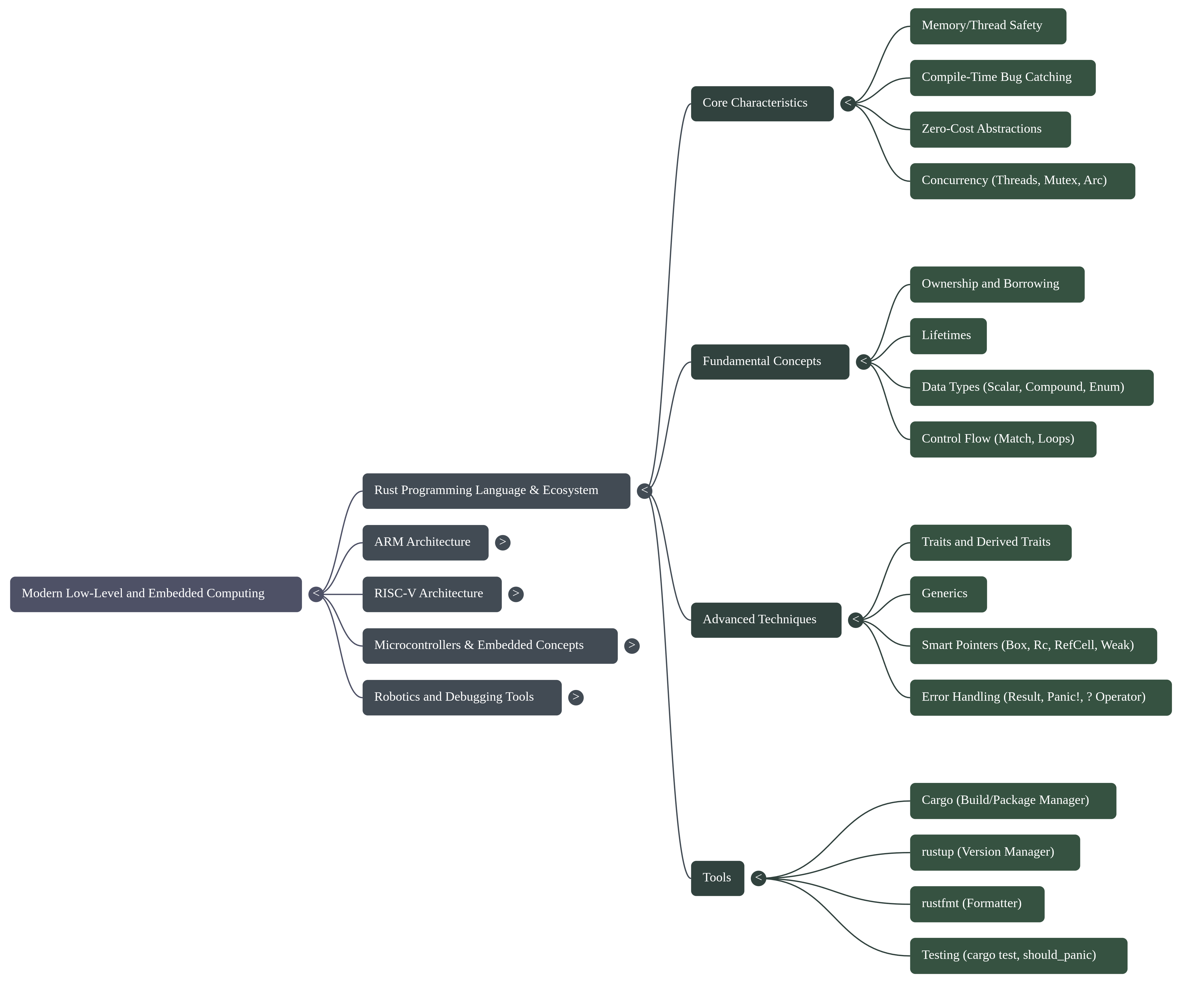
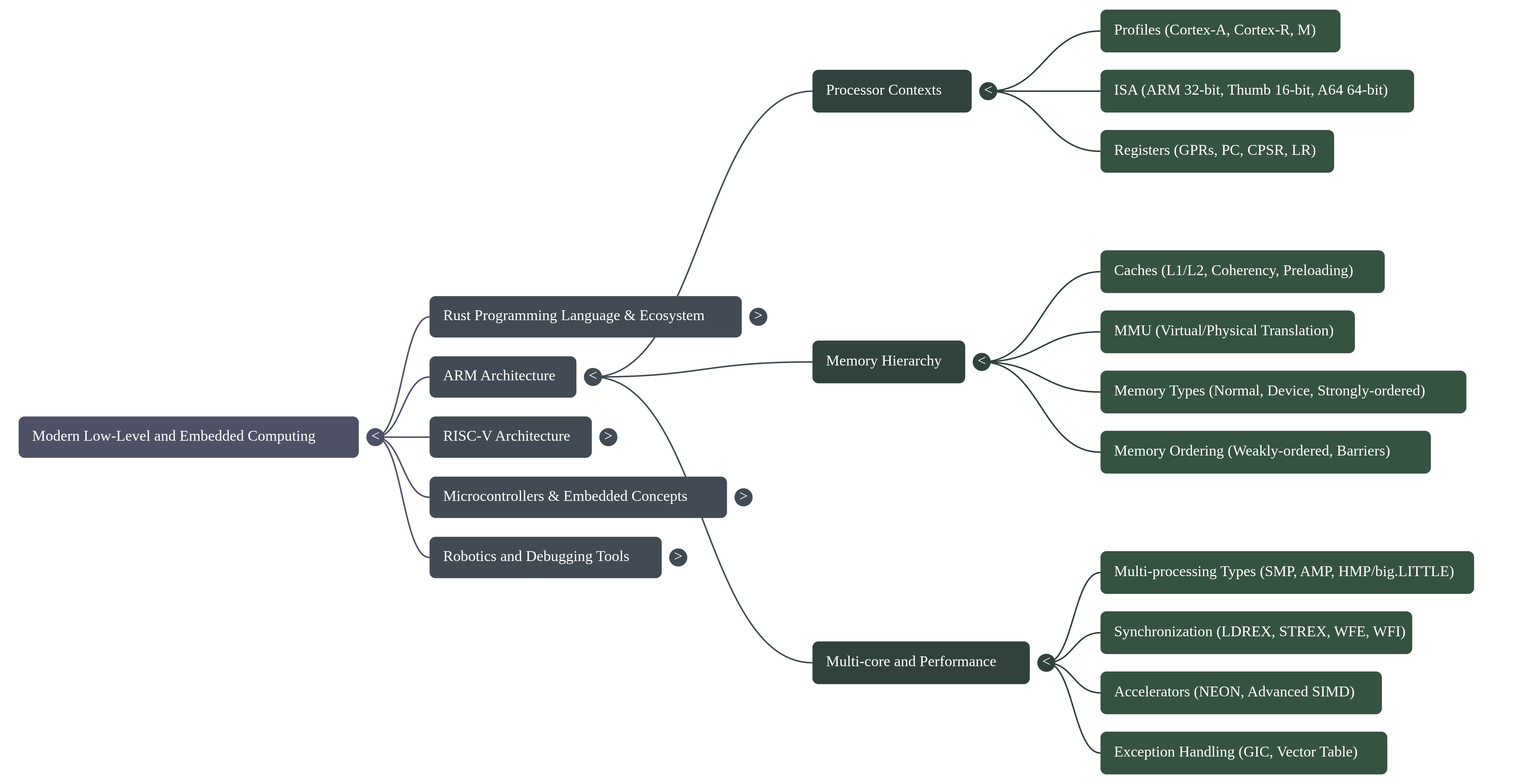
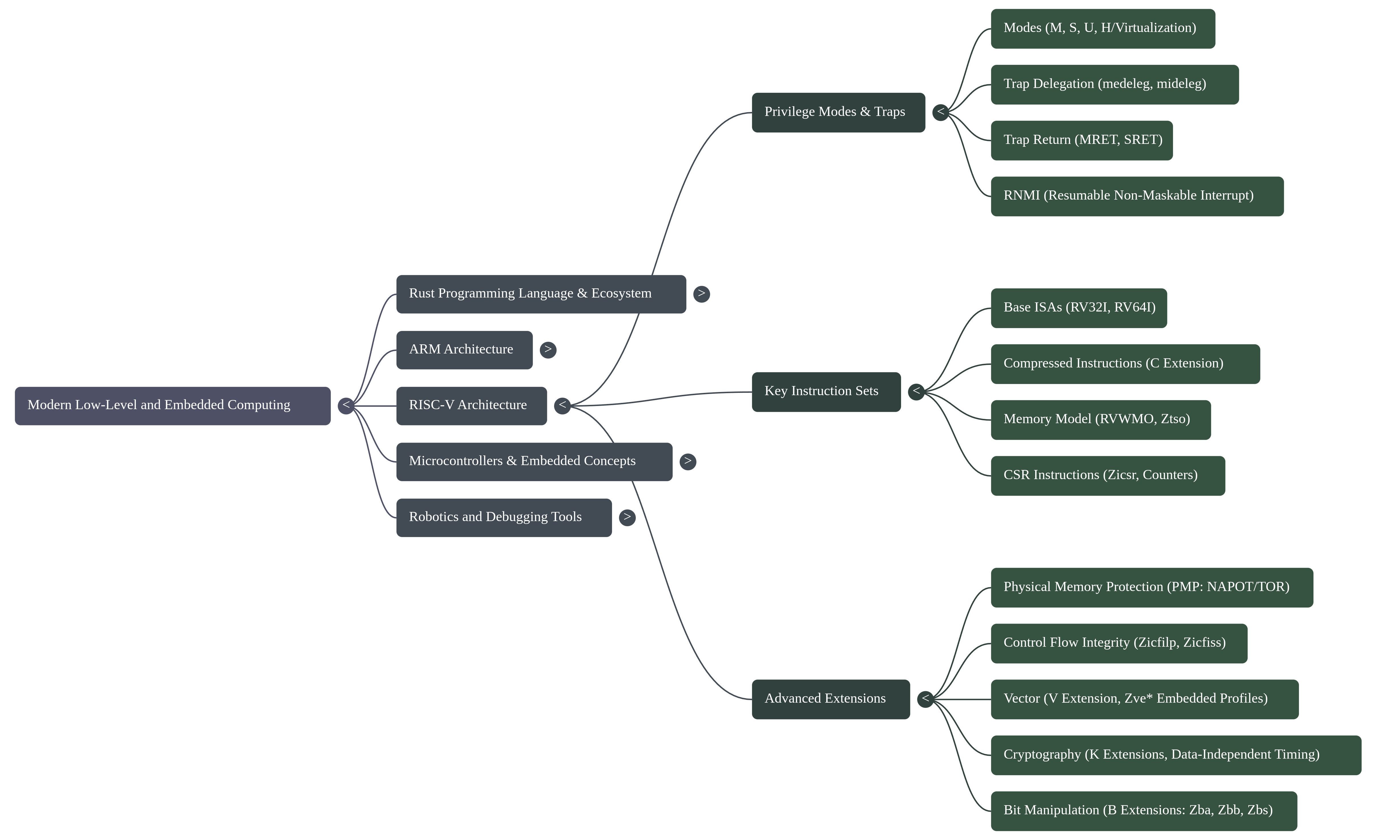
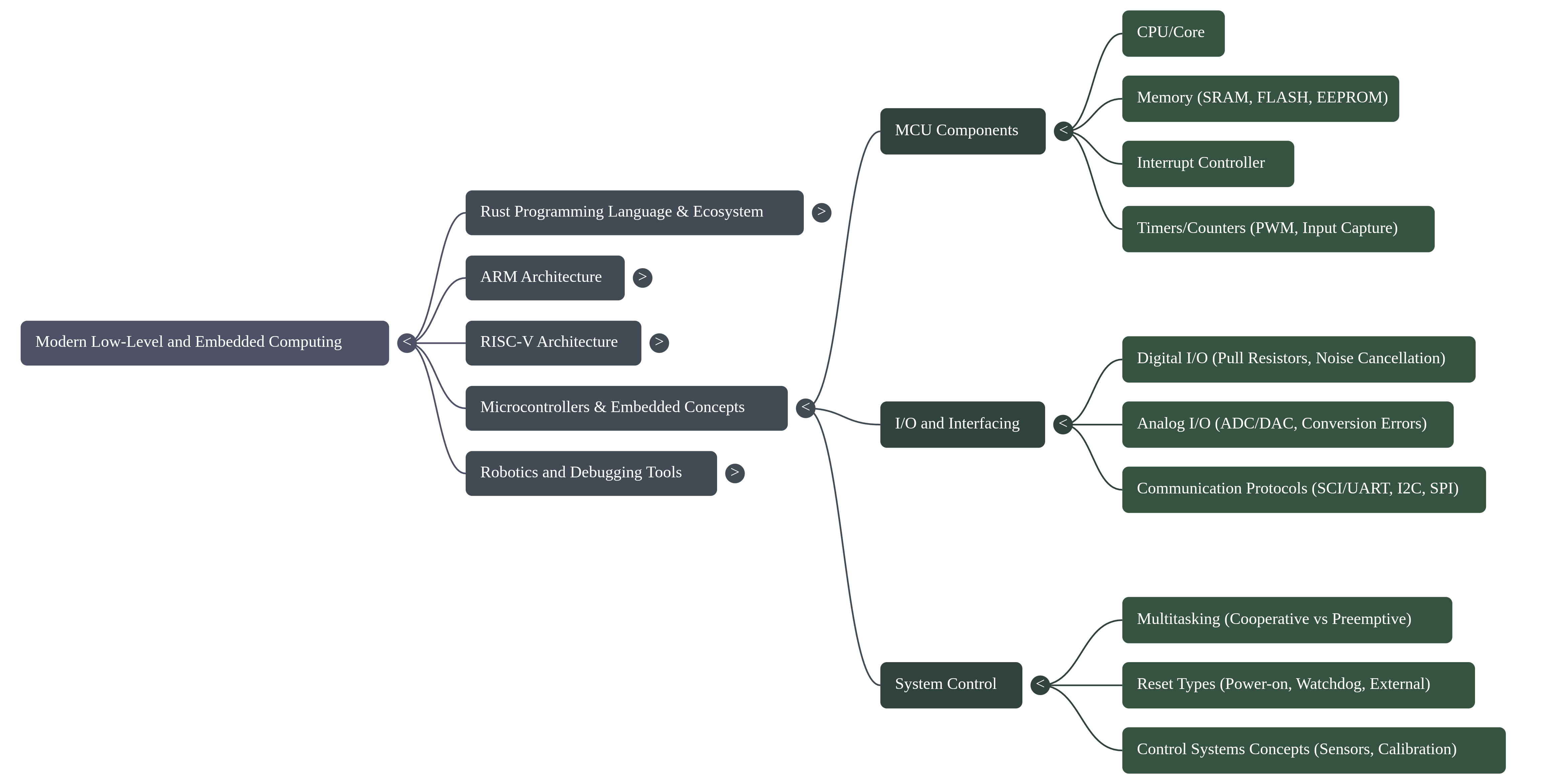
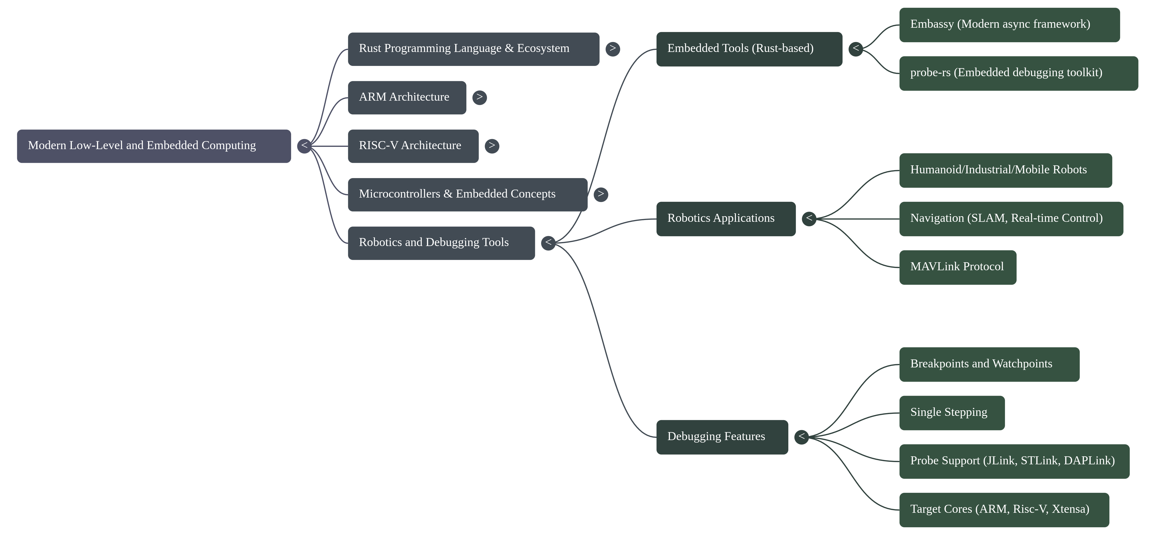
Modern embedded systems development is strained by a fundamental tension: while hardware complexity explodes, the traditional C/C++ development paradigm offers insufficient compile-time guarantees against critical memory and concurrency failures. A fundamental paradigm shift is underway to address this, moving away from legacy approaches toward a powerful synergy between advanced hardware architectures and modern, memory-safe programming languages. This shift is defined by the adoption of high-performance languages like Rust, known for its core tenets of building reliable and efficient software, in concert with sophisticated processor architectures such as ARM and RISC-V.
Frameworks like Embassy are emerging to leverage this new paradigm, enabling developers to write safe, correct, and energy-efficient embedded code using Rust's advanced async capabilities. The strategic application of these modern language features provides compile-time guarantees against entire classes of common and dangerous bugs, such as memory errors and data races, which have historically plagued embedded development.
This report analyzes the core technical pillars that underpin this modern paradigm: foundational safety, hardware abstraction, performance optimization, and the developer ecosystem. It will deconstruct the implementation methodologies that bring these pillars to life and examine the inherent challenges and limitations that engineers must navigate in this demanding field.
2. Core Technical Pillars
The modern embedded paradigm is built upon several foundational technical pillars that collectively address the core challenges of safety, abstraction, and performance. This new model does not treat these concerns as separate; instead, it integrates them through a combination of language design, hardware architecture, and a robust developer ecosystem. This section deconstructs these essential pillars.
2.1 Pillar 1: Foundational Safety and Reliability
In embedded systems—where software failure can lead to equipment damage or risk to human life—memory and concurrency safety are paramount. The adoption of modern languages is driven by the ability to provide these safety guarantees without sacrificing performance. Rust, in particular, provides these guarantees at compile time, eliminating entire classes of bugs before the code is ever deployed to a device.
- Memory Safety: Rust's ownership and borrowing model is a cornerstone of its safety guarantees. It enforces strict rules at compile time that ensure there is only one owner of a piece of data, preventing common errors like dangling pointers, buffer overflows, and use-after-free vulnerabilities. Crucially, this is achieved without a garbage collector, making it perfectly suited for resource-constrained, systems-level work where deterministic performance is essential.
- Thread Safety: With the rise of multi-core processors in embedded systems, managing concurrency safely is critical. Rust's type system extends its ownership model to multithreading, preventing data races at compile time. This compile-time guarantee is a revolutionary departure from traditional approaches that rely on runtime detection or developer discipline, which are inadequate for the complex Symmetric Multi-Processing (SMP) systems now common in embedded applications.
- Robust Error Handling: Traditional error handling, often relying on null
pointers or error codes, can be easily overlooked by developers. Rust uses a
Result<T, E>enum, which forces the developer to explicitly handle the possibility of failure. This ensures that errors are acknowledged and managed, leading to more robust and predictable software.
2.2 Pillar 2: Abstraction and Direct Hardware Control
Embedded systems engineering presents a unique duality: developers need high-level abstractions to manage complexity, but also require direct, low-level control over the underlying hardware. The modern paradigm addresses this by providing tools that can operate at both levels of abstraction, built upon a deep understanding of the hardware components.
-Microcontroller Architecture: A microcontroller (MCU) is a self-contained computer on a single chip, designed for control tasks. It integrates a processor core (CPU), memory, I/O peripherals, timers, and an interrupt controller. This integration allows it to operate stand-alone, directly interfacing with its environment through general-purpose I/O pins. -Processor Cores: The dominant architectures in this space are ARM and RISC-V. Both are based on Reduced Instruction Set Computer (RISC) principles and are load/store architectures, meaning that arithmetic and logic instructions operate on registers, and only specific load and store instructions access memory. The ARM architecture is further divided into profiles tailored for different applications, such as the Cortex-A series for high-performance applications and the Cortex-R series for real-time systems. These cores can operate in different execution states, such as the 32-bit AArch32 or the 64-bit AArch64 state. This profile-based specialization allows hardware to be precisely tailored to an application's cost, power, and performance envelope, ranging from high-throughput application processors to fault-tolerant, deterministic real-time controllers. -Memory Systems: Embedded systems utilize a hierarchy of memory types. This includes fast but volatile Static RAM (SRAM) for data, and non-volatile Flash or EEPROM for program code and constants. High-performance systems, particularly in the real-time Cortex-R family, also feature Tightly Coupled Memory (TCM) for deterministic, low-latency access—a critical feature for hard real-time tasks where the non-deterministic latency of cache hierarchies is unacceptable. More complex Cortex-A processors include multi-level caches (L1/L2) and a Memory Management Unit (MMU) to translate virtual addresses generated by the core into physical memory addresses. -Peripherals and Communication: Software must directly control a wide range of on-chip peripherals to interact with the outside world. Common peripherals include General-Purpose Input/Output (GPIO) pins, Pulse Width Modulation (PWM) for controlling motors, and Analog-to-Digital Converters (ADC) for reading sensors. Communication is handled via standard protocols like I2C, SPI, and UART.
2.3 Pillar 3: Performance and Optimization
Performance and energy efficiency are non-negotiable requirements in most embedded applications, from battery-powered IoT devices to real-time robotics controllers. The modern paradigm achieves high performance through a combination of efficient hardware features and software abstractions that compile down to optimized machine code.
-Instruction Set Architecture (ISA): The RISC principles underlying both ARM and RISC-V contribute to efficient execution. ISAs are designed for optimal performance and code density. For example, the ARM architecture includes the 32-bit ARM instruction set and the more compact 16/32-bit Thumb instruction set to reduce memory footprint. The A64 instruction set provides a clean, fixed-length instruction set for 64-bit computing. -Advanced SIMD and Vector Processing: Modern embedded processors feature powerful Single Instruction, Multiple Data (SIMD) capabilities to accelerate operations on large datasets. ARM's NEON technology and the RISC-V Vector ("V") extension allow a single instruction to perform an operation on multiple data points simultaneously. This is highly effective for tasks like media codecs, digital signal processing, and the matrix multiplication routines common in robotics and machine learning. -_Software Abstractions: Modern languages like Rust provide "zero-cost abstractions," allowing developers to write high-level, expressive code that compiles down to machine code as fast as manually written low-level code. Features like async programming, central to frameworks like Embassy, enable the creation of highly concurrent applications that are also energy-efficient by allowing tasks to yield control and the processor to enter low-power sleep states while awaiting I/O events, a stark contrast to the power-inefficient busy-waiting or thread-based context switching required by traditional blocking models.
2.4 Pillar 4: A Modern Developer Ecosystem
Developer productivity and code quality are heavily influenced by the toolchain. The modern embedded paradigm is supported by a comprehensive and integrated ecosystem of tools that streamline the entire development lifecycle, from project creation to on-target debugging.
-Project Management & Build System: Rust's build system and package manager,
Cargo, automates many of the most tedious development tasks. It handles
downloading library dependencies, compiling code, running tests, and building
the final binary, providing a consistent and reproducible build process for any
project.
-Code Quality and Formatting: To ensure code consistency across teams and
projects, tools like rustfmt automatically format Rust code according to a
standard style. This eliminates debates over formatting and allows developers to
focus on the logic of their applications.
-_Debugging and Flashing: Modern debugging tool-sets like probe-rs provide a
unified interface for on-chip debugging. Written in Rust, probe-rs can
connect to a wide variety of debug probes and interface with both ARM and RISC-V
cores. Its capabilities include reading and writing memory, halting and stepping
through code, managing breakpoints, and flashing binaries to the target device.
This toolkit provides a modern, unified software interface to the low-level
debug hardware, such as JTAG and SWD interfaces, that are physically present on
the microcontrollers.
3. Methodologies and Implementation
The practical implementation of this paradigm hinges on methodologies that skillfully combine Rust's high-level features with direct hardware control. Developers write expressive and safe application logic using a rich feature set, while simultaneously employing sophisticated optimization and debugging techniques to create robust and efficient applications.
-Leveraging High-Level Language Features: The methodology hinges on the
strategic application of Rust's features to solve long-standing embedded
problems. The async/.await syntax, central to frameworks like Embassy, is used
to build highly concurrent applications that are efficient and easier to reason
about than traditional callback-based or threaded models. Traits are used to
create powerful abstractions, while the Result<T,E> enum and the ? operator
provide a clean and robust mechanism for propagating and handling errors.
-Interfacing with Hardware: Direct hardware control is fundamental to embedded
programming. This involves writing to specific memory-mapped registers to
configure and control peripherals like GPIOs and timers. Interrupts, which
signal events from hardware, are handled by writing Interrupt Service Routines
(ISRs) that execute when an event occurs. These low-level operations are
combined with higher-level multitasking concepts to manage the overall system
behavior.
-Applying Performance Optimization: To meet strict performance targets,
developers explicitly leverage advanced hardware features. For computationally
intensive tasks like matrix multiplication, NEON intrinsics are used to issue
SIMD instructions directly from high-level code. While the source example
demonstrates this technique in C, Rust provides equivalent access to these
low-level hardware capabilities. Achieving maximum performance often requires
careful data layout, such as de-interleaving data structures to ensure that
related data is contiguous in memory for vector processing. Compilers are guided
using specific flags (e.g., -mcpu to target a specific core, -mfpu to enable
floating-point hardware) to generate the most optimized code for the target
hardware.
-Debugging and Verification: The debugging workflow is streamlined by modern
tools. A developer uses probe-rs, either through its command-line interface or
a VS Code extension, to flash new firmware onto a target microcontroller. From
there, they can perform standard debugging tasks such as setting breakpoints,
stepping through code instruction-by-instruction, and inspecting memory and
variable states. In addition to on-target debugging, Rust's built-in testing
framework (cargo test) enables developers to write and run unit tests for
business logic, ensuring correctness before deployment to hardware.
4. Challenges and Limitations
Despite the significant advancements offered by the modern paradigm, developing for embedded systems involves navigating inherent complexities, trade-offs, and limitations. The tight coupling of software with hardware means that developers must contend with issues that are abstracted away in higher-level application development.
-Inherent Hardware Complexity: Modern processors, while powerful, introduce
low-level complexities that software must manage. For instance, many ARM cores
have a weakly-ordered memory model, meaning that memory operations can be
reordered by the hardware. To ensure correctness, for instance when
synchronizing with a peripheral or another core, developers must insert explicit
memory barrier instructions (like the Data Synchronization Barrier, DSB) to
enforce a specific order of memory operations. In multi-core systems,
maintaining cache coherency—ensuring all cores have a consistent view of
memory—is a significant and complex challenge.
-Resource Constraints: Embedded systems are defined by their constraints. They
operate with limited memory (SRAM and Flash), tight power consumption budgets,
and finite processing power. These constraints dictate every aspect of software
design, from the choice of algorithms and data structures to the implementation
style, forcing a constant focus on efficiency.
-Tooling and Abstraction Gaps: Even modern tools have limitations. For
example, rustfmt is an excellent code formatter but cannot handle every
possible edge case in Rust's syntax. Furthermore, educational materials often
deliberately avoid deep, complex topics like linker scripts—which control how
compiled code is laid out in memory—because they remain a significant hurdle for
many developers, indicating a gap in user-friendly abstraction.
-Cross-Platform Portability: Writing portable embedded software is a
non-trivial task. Porting code between different processor architectures
requires careful management of endianness (the byte order of data in memory),
instruction set differences, and assumptions about memory ordering models. Code
that works correctly on one platform may fail subtly on another if these details
are not properly handled.
-_Developer Learning Curve: The powerful features of modern systems and
languages come with a corresponding learning curve. Rust, in particular, is
known for its steep initial learning curve, as developers must internalize the
rules of its ownership and borrow checking system. While this system is the
source of Rust's safety guarantees, it represents a significant conceptual shift
for programmers accustomed to other languages.
5. Conclusion
This report has analyzed the paradigm shift in modern embedded systems, characterized by the powerful synergy between the compile-time safety guarantees of Rust and the advanced computational capabilities of ARM and RISC-V hardware. The paradigm shift is therefore not merely an adoption of new tools, but a fundamental re-design of the developer's relationship with the hardware. It replaces a paradigm of manual, error-prone memory management and concurrency control with one where safety guarantees are an automated, architectural first principle.
This shift is critical, as it is the primary enabler for reliably building the complex, multi-core, and safety-critical systems that define the next generation of embedded computing. It allows engineers to develop increasingly sophisticated systems—from low-power microcontrollers to complex robotics platforms—with a higher degree of confidence in their correctness and reliability. While significant challenges related to hardware complexity and resource constraints remain, the maturing ecosystem is making this power more accessible. Frameworks like Embassy provide high-level abstractions for concurrency, while toolchains like probe-rs unify and simplify the critical process of on-target debugging.
Looking forward, the continued convergence of software safety and hardware performance promises to further accelerate innovation. As these tools and methodologies become more widespread, engineers are better equipped to build the next generation of intelligent, reliable, and efficient embedded systems that are foundational to our technological world.